Naive Bayes
Basic Ideas
Supervised Learning
Problem Setting:
- Set of possible instances: $X$
- Unknown target function (concept): $f: X\rightarrow Y$
- Set of hypotheses (hypothesis class): $H = {h\lvert h:X\rightarrow Y}$
Given:
- Training set of instances of unknown target function $f$, $(x^{(1)}, y^{(1)})$, $(x^{(2)}, y^{(2)})$, … , $(x^{(m)}, y^{(m)})$.
Output:
- Hypothesis $h\in H$ that best approximates target function.
Discriminative Approaches
- Hypothesis $h \in H$ directly predicts the label $y$ given the features $x$
\(y = h(x) \,\,\,or\,\,\,p(y\lvert x)=h(x)\) - Define a loss function $L(h)$ and find hypothesis with minimum loss.
- Probabilistic model is a special case, like finding MLE or MAP.
- Example: Linear regression
\(\begin{aligned} &h_{\theta}(x) = \langle x,\theta\rangle \\ &L(h_{\theta} = \frac{1}{m}\sum_{i=1}^m(h_{\theta}(x^{(i)}) - y^{(i)})^2 \end{aligned}\)
Generative Approaches
- Hypothesis $h\in H$ specifies a generative probabilistic story for how the full data (x,y) was created \(h(x,y)=p(x,y)\)
- Pick a hypothesis by Maximum Likelihood Estimation (MLE) or Maximum A Posteriori (MAP).
- Example: Roll a weighted die
- Weights for each side($\theta$) define how the data are generated.
- Use MLE on the training data to learn $\theta$
Maximum Likelihood Estimation (MLE) and Maximum A Posteriori (MAP)
MLE vs. MAP Suppose we have data $D = {x^{(i)} }^N_{i=1}$,
\[\begin{aligned} &\theta^{MLE} = \arg\max_\theta \prod_{i=1}^Np(x^{(i)}\lvert \theta) \\ &\theta^{MAP} = \arg\max_\theta \prod_{i=1}^Np(x^{(i)}\lvert \theta)p(\theta) \end{aligned}\]To be noticed, the $p(\theta)$ in MAP is the prior distribution.
Example: MLE of Exponential Distribution
- First write the log-likelihood of the sample, that is
\(\begin{aligned} \mathcal{l}(\lambda) &= \sum_{i=1}^N\log f(x^{(i)})\\ &= N\log(\lambda) - \lambda \sum_{i=1}^N x^{(i)} \end{aligned}\) - Compute first derivative, set to zero, solve for $\lambda$.
\(\begin{aligned} \frac{\partial\mathcal{l}(\lambda)}{\partial\lambda} &= \frac{N}{\lambda} - \sum_{i=1}^N x^{(i)} = 0 \\ &\Rightarrow \lambda^{MLE} = \frac{N}{\sum^N_{i=1}x^{i}} \end{aligned}\)
Naive Bayes
Generic Naive Bayes Model
- Support: Depends on the choice of event model, $P(X_k\lvert Y)$.
- Model: Product of prior and the event model.
\(\begin{aligned} P(X,Y) &= P(Y)P(X\lvert Y) \\ &= P(Y)\prod_{k=1}^KP(x_k\lvert Y) \end{aligned}\) - Training: Find the class-conditional MLE parameters
- For $P(Y)$, we find the MLE using all the data. For each $P(x_k\lvert Y)$ we condition on the data with the corresponding.
- Classification: Find the class that maximizes the posterior
\(\begin{aligned} \hat{y} &= \arg\max_y p(y\lvert X)) \,\,\,(Posterior)\\ &= \arg\max_y\frac{p(X\lvert y)p(y)}{p(x)} \,\,\,(P(x) \,\,\,is\, fixed)\\ &= \arg\max_y p(X\lvert y)p(y) \end{aligned}\)
Bayesian Network
Bayesian Networks
Overview
- A Bayesian Network (BN) consists of a Directed Acyclic Graph (DAG) and a set of conditional probability distributions.
- In a DAG
- Each node denotes a random variable.
- Each edge from $X$ to $Y$ represents that $X$ directly influences $Y$.
- Formally: each variable X is independent of its non-descendants given its parents.
- Each node $X$ has a conditional probability distribution (CPD) representing $P(X\lvert Parents(X))$.
- BN provides a compact representation of a joint probability distribution, using chain rule.
\(P(X_1, \cdots X_n) = P(X_1)\prod_{i=2}^n P(X_i\lvert Parents(X_i))\)
Advantages
- Captures independence and conditional independence where they exist.
- Encodes the relevant portion of the full joint among variables where dependencies exist.
- Uses a graphical representation which lends insight into the complexity of inference.
The inference task in Bayesian networks
Given: values for some variables in the network (evidence), and a set of query variables
Do: Compute the posterior distribution over the query variables.
- Variables that are neither evidence variables nor query variables are hidden variables.
- The BN representation is flexible enough that any set can be the evidence variables and any set can be the query variables.
- Inference by enumeration is an exact method (i.e. it computes the exact answer to a given query).
- It requires summing over a joint distribution whose size is exponential in the number of variables.
- In many cases we can do exact inference efficiently in large networks
- key insight: save computation by pushing sums inward.
- In general, the Bayes net inference problem is NP-hard.
- There are also methods for approximate inference - these fer an answer which is “close”.
- In general, the approximate inference problem is NP-hard also, but approximate methods work well for many real-world problems.
The parameter learning task in Bayesian networks
- Given: a set of training instances, the graph structure of a BN.
- Do: infer the parameters of the CPDs.
The structure learning task in Bayesian networks
- Given: a set of training instances.
- Do: infer the graph structure (and perhaps the parameters of the CPDs too)
Parameter learning and MLE
Overview
- Maximum Likelihood Estimation (MLE)
- Given a model structure (e.g. a Bayes net graph) $G$ and a set of data $D$.
- Set the model parameters $\theta$ to maximize $P(D\lvert G, \theta)$.
- i.e. make the data $D$ look as likely as possible under the model $P(D\lvert G, \theta)$
Parameter learning and MAP
Overview
- Instead of estimating parameters strictly from the data,
we could start with some prior belief for each. - Laplace Estimates
- $n_v$ represents the number of occurrences of value $v$. \(P(X=x) = \frac{n_x+1}{\sum_{v\in Values(X)}(n_v+1)}\)
- M-estimates
- $p_x$ prior probability of value $x$
- Number of “Virtual” instances
\(P(X=x) = \frac{n_x+p_xm}{\sum_{v\in Values(X)}(n_v) + m}\)
Missing Data
- Hidden variables; Values missing at random
- these are the cases we’ll focus on
- one solution: try impute the values
- Values missing systematically
- may be sensible to represent “missing” as an explicit feature value
Imputing missing data with EM
Overview
Given:
- Data set with some missing values.
- Model structure, initial model parameters.
Repeat until convergence:
- Expectation (E) step: using current model, compute expectation over missing values
- Maximization (M) step: update model parameters with those that maximize probability of the data (MLE or MAP)
- i.e. Re-estimate probabilities using expected counts.
Covergence of EM
- E and M steps are iterated until probabilities converge
- Will converge to a maximum in the data likelihood (MLE or MAP)
- The maximum may be a local optimum.
- The optimum found depends on starting conditions (initial estimated probability parameters)
Learning structure + parameters
- Number of structures is superexponential in the number of variables
- Finding optimal structure is NP-complete problem
- Two common options:
- Search very restricted space of possible structures (e.g. networks with tree DAGs)
- Use heuristic search (e.g. sparse candidate)
The Chow-Liu algorithm
Overview
- Learns a BN with a tree structure that maximizes the likelihood of the training data
- Notice, Chow-Liu algorithm always has a complete graph.
- Algorithm:
- Compute weight $I(X_i,X_j)$ of each possible edge $(X_i, X_j)$
- Use mutual information to calculate edge weights. $I(X,Y) = \sum_{x\in X}\sum_{y\in Y}P(x,y)\log_2\frac{P(x,y)}{P(x)P(y)}$ \(\begin{aligned} I(X; Y) &= \sum_{x\in\mathcal{X}, y\in\mathcal{Y}}P_{(X,Y)}(x,y)\log{\frac{P_{(X,Y)}(x,y)}{P_X(x)P_Y(y)}} \\ &= \sum_{x\in\mathcal{X}, y\in\mathcal{Y}}P_{(X,Y)}(x,y)\log{\frac{P_{(X,Y)}(x,y)}{P_X(x)}} - \sum_{x\in\mathcal{X}, y\in\mathcal{Y}}P_{(X,Y)}(x,y)\log{P_Y(y)} \\ &= \sum_{x\in\mathcal{X}, y\in\mathcal{Y}}P_X(x)P_{Y\lvert X=x}(y)\log{P_{Y\lvert X=x}(y)} - \sum_{x\in\mathcal{X}, y\in\mathcal{Y}}P_{(X,Y)}(x,y)\log{P_Y(y)} \\ &= \sum_{x\in\mathcal{X}}P_X(x)(\sum_{y\in\mathcal{Y}}P_{Y\lvert X=x}(y)\log{P_{Y\lvert X=x}(y)}) - \sum_{y\in\mathcal{Y}}(\sum_{x}P_{X,Y}(x,y))\log{P_Y(y)} \\ &= -\sum_{x\in\mathcal{X}}P(x)H(Y\lvert X=x) - \sum_{y\in\mathcal{Y}}P_Y(y)\log{P_Y(y)}\\ &= -H(Y\lvert X) + H(Y) \\ &= H(Y) - H(Y\lvert X) \end{aligned}\)
- Find maximum weight spanning tree (MST)
- A maximal-weight tree that connects all vertices in a graph.
- Prim’s algorithm and Kruskal’s algorithm. Go review CS400.
- Assign edge directions in MST.
- Pick a node for the root, and assign edge directions.
- Compute weight $I(X_i,X_j)$ of each possible edge $(X_i, X_j)$
Heuristic search for structure learning
- Each state in the search space represents a DAG Bayes net structure.
- To instantiate a search approach, we need to specify
- Scoring function
- State transition operators
- Search algorithm
Scoring Function
Decomposability
When the appropriate priors are used, and all instances in D are complete, the scoring function can be decomposed as follows
This decomposability allows us to
- Score a network by summing terms over the nodes in the netwrok.
- Efficiently score changes in a local search procedure.
Structure learning
One general approach for BN structure search
where the $f(m)\lvert \theta_G\lvert$ is the complexity penalty.
Akaike Informtion Criterion (AIC)
Bayesian Informtion Criterion (AIC)
\[f(m) = \frac{1}{2}\log (m)\]Structure search operators
- Add an edge
- Delete an edge
- Reverse an edge
Bayesian Network Search
Algorithm 1: Hill-Climbing
given: data set $D$, initial network $B_0$
Pseudocode:
$i=0$
$B_{best} \leftarrow B_0$
while stopping criteria not met
{
$\quad$for each possible operator application $\alpha$
$\quad${
$\quad\quad${
$\quad\quad\quad B_{best} \leftarrow apply(\alpha,B_i)$
$\quad\quad\quad$if $score(B_{new})>score(B_{best})$
$\quad\quad\quad\quad B_{best} \leftarrow B_{new}$
$\quad\quad$}
$\quad$++$i$
$\quad$$B_i \leftarrow B_{best}$
}
return $B_i$
Algorithm 2: the Sparse Candidate algorithm
given: data set $D$, initial network $B_0$, parameter $k$
Pseudocode:
$i=0$
repeat
{
$\quad$++$i$
$\quad$// restrict step
$\quad$select for each variable $X_j$ a set $C_j^i$ of candidate parents $(\lvert C_j^i\lvert \leq k)$
$\quad$// maximize step
$\quad$find network $B_i$ maximizing score among networks where $\forall X_j, Parents(X_j) \subseteq C_j^i$
} until convergence
return $B_i$
The restrict step in Sparse Candidate Algorithm
To identify candidate parents in the first iteration, can compute the mutual information between pairs of variables, $I(X,Y) = \sum_{x\in X}\sum_{y\in Y}P(x,y)\log_2\frac{P(x,y)}{P(x)P(y)}$
Kullback-Leibler (KL) divergence provides a distance measure between two distributions, $P$ and $Q$
\[D_{KL}(P(X)\lvert Q(X)) = \sum_xP(x)\log\frac{P(x)}{Q(x)}\]KL divergence can be used to assess the discrepancy between the network’s $P_{net}(X, Y)$ and the empirical $P(X, Y)$.
\[M(X,Y) = D_{KL}(P(X,Y)\lvert P_{net}(X,Y))\]Notice, $P_{net}(X,Y)$ can be estimated through sampling from the network.
given: data set $D$, initial network $B_0$, parameter $k$
Pseudocode of restrict step:
for each variable $X_j$
{
$\quad$ calculate $M(X_j,X_l)$ for all $X_j \neq X_l$ such that $X_l \notin Parents(X_j)$
$\quad$ choose highest ranking $X_l, \cdots X_{k-s}$ where $s=\lvert Parents(X_j)\lvert$
$\quad$ // include current parents in candidate set to ensure monotonic
$\quad$ // improvement in scoring function
$\quad$ $C_j^i = Parents(X_j) \cup X_1 … X_{k-s}$
}
return ${ C_j^i }$ for all $X_j$
The maximize step in Sparse Candidate
- Hill-climbing search with add-edge, delete-edge, reverse-edge operators.
- Test to ensure that cycles aren’t introduced into the graph.
Bayes nets for classification
Previously discussed method are mainly unsupervised. However, BN learning can be also used for a standard supervised task (learn a model to predict $Y$ given $X_1,… , X_n$).
- One very simple BN approach for supervised tasks is naïve Bayes
- In naïve Bayes, we assume that all features $X_i$ are conditionally independent given the class $Y$
Naive Bayes
Learning:
- Estimate $P(Y = y)$ for each value of the class variable $Y$
- Estimate $P(X_i=x \lvert Y = y)$ for each $X_i$
Classification: use Bayes’ Rule
\[\begin{aligned} P(Y = y\lvert x) &= \frac{P(y)P(x\lvert y)}{\sum_{y'}P(x\lvert y')} \\ &= \frac{P(y)\prod_{i=1}^nP(x_i\lvert y)}{\sum_{y'}(P(y')\prod_{i=1}^nP(x_i\lvert y'))} \end{aligned}\]The Tree Augmented Network (TAN) algorithm
- Learns a tree structure to augment the edges of a naïve Bayes network.
- Algorithm:
- Compute weight $I(X_i,X_j\lvert Y)$ for each possible edge $(X_i,X_j)$ between features
- Find maximum weight spanning tree (MST) for graph over $X_l … X_n$
- Assign edge direction in MST
- Construct a TAN model by adding node for $Y$ and an edge from $Y$ to each $X_i$
- Condition mutual information
\(I(X_i,X_j\lvert Y) = \sum_{x_i\in X_i}\sum_{x_j\in X_j}\sum_{y\in Y}P(x_i, x_j, y)\log_2\frac{P(x_i,x_j\lvert y)}{P(x_i\lvert y)P(x_j\lvert y)}\)
Tan Network Example
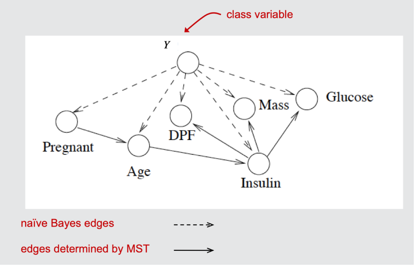
TAN vs. Chow-Liu
- TAN is focused on learning a Bayes net specifically for classification problems
- The MST includes only the feature variables (the class variable is used only for calculating edge weights)
- Conditional mutual information is used instead of mutual information in determining edge weights in the undirected graph
- The directed graph determined from the MST is added to the $Y \rightarrow X_i$ edges that are in a naïve Bayes network.