Back Propagation

Back Propagation

Perceptrons

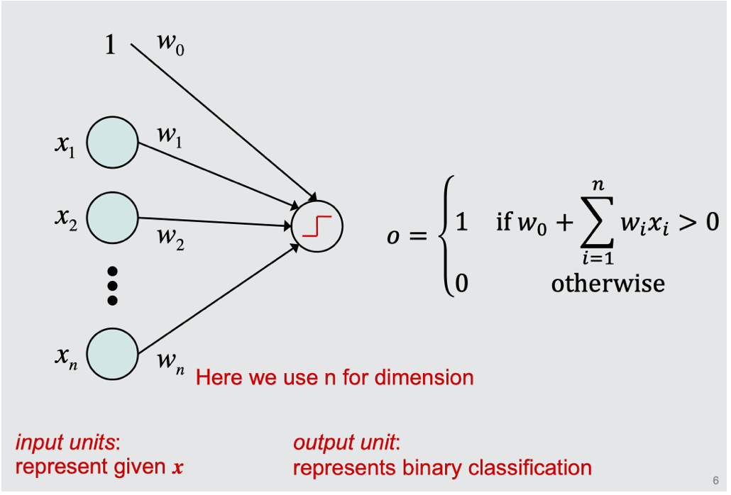
A toy model of perceptrons

The perceptron training rule

1. Initialize weights $w=0$
2. Iterate through training instances until convergence
   1. Calculate the output for the given instances.
      \(o = \begin{cases} 1 \,\, if\,\,w_0 + \sum_{i=1}^n w_ix_i>0 \\ 0 \,\,o.w. \end{cases}\)
   2. Update each weight
      \(\begin{aligned} \Delta w_i = (y-o)x_i \\ w_i \leftarrow w_i + \Delta w_i \end{aligned}\)

Remarks
A multilayer perceptron can represent XOR.

Multiple Layer Neural Networks

Components

• Representations:
  • Input
  • Hidden variables
• Layers/weights:
  • Hidden layers
  • Output layer

Typical activation function

• Threshold function
  \(t(z) = \mathbb{1}[z\geq 0]\)
• Sigmoid function
  \(\sigma = \frac{1}{1+e^{-z}}\)
• Tanh function
  \(\tanh(z) = 2\sigma(2z)-1\)
• ReLU function
  • Standard ReLU \(ReLU(z) = max\{z,0\}\)
  • Generalization of ReLU
    \(gReLU(z) = max\{z,0\} + \alpha\min\{z,0\}\)
    • Leaky-ReLU function
      \(Leaky-ReLU(z) = max\{z,0\} + 0.01\min\{z,0\}\)
    • Parametric-ReLU function
      $\alpha$ is learnable.

Backpropagation

Gradient descent in weight space
Overview
Given a training set $D = {(x^{(1)}, y^{(1)}), \cdots,(x^{(m)}, y^{(m)})}$, we can specify an error measure that is a function of the weight vector $w$

\[E(w) = \frac{1}{2}\sum_{d\in D}(y^{(d)} - o^{(d)})^2\]

Gradient Descent Algorithm
Gradient descent is an iterative process aimed at finding a minimum in the error surface
In each iteration:

1. Current weights define a point in this space.
2. Find direction in which error surface descends most steeply.
3. Take a step (i.e. update weights) in that direction.

Mathematics Representation

1. Calculate the gradient of $E$

   \[\nabla E(w) = [\frac{\partial E}{\partial w_0}, \frac{\partial E}{\partial w_1}, \cdots, \frac{\partial E}{\partial w_n}]\]

2. Take a step in the opposite direction

   \[\begin{aligned} &\Delta w=-\eta \nabla E(w) \\ &\Delta w_i=-\eta \frac{\partial E}{\partial w_i} \end{aligned}\]

Batch neural network training
Given: network structure and a training set $D = {(x^{(1)}, y^{(1)}), \cdots,(x^{(m)}, y^{(m)})}$
Pseudocode
initialize all weights in $w$ to small random numbers
until stopping criteria met do
$\quad$ initialize the error $E(w) = 0$
$\quad$ for each $(x^{(d)}, y^{(d)})$ in the training set
$\quad\quad$ input $x^{(d)}$ to the network and compute output $o^{(d)}$
$\quad\quad$ increment the error $E(w) = E(w) + \frac{1}{2}(y^{(d)} - o^{(d)})^2$
$\quad$ calculate the gradient

\[\nabla E(w) = [\frac{\partial E}{\partial w_0}, \frac{\partial E}{\partial w_1}, \cdots, \frac{\partial E}{\partial w_n}]\]

$\quad$ Update the weights

\[\Delta w = -\eta \nabla E(w)\]

Online neural network training (stochastic gradient descent)
Given: network structure and a training set $D = {(x^{(1)}, y^{(1)}), \cdots,(x^{(m)}, y^{(m)})}$
Pseudocode
initialize all weights in $w$ to small random numbers
until stopping criteria met do
$\quad$ for each $(x^{(d)}, y^{(d)})$ in the training set
$\quad\quad$ input $x^{(d)}$ to the network and compute output $o^{(d)}$
$\quad\quad$ calculate the error $E(w) = \frac{1}{2}(y^{(d)} - o^{(d)})^2$
$\quad\quad$ calculate the gradient

\[\nabla E(w) = [\frac{\partial E}{\partial w_0}, \frac{\partial E}{\partial w_1}, \cdots, \frac{\partial E}{\partial w_n}]\]

$\quad$$\quad$ Update the weights

\[\Delta w = -\eta \nabla E(w)\]

Online vs. batch training

• Standard gradient descent (batch training): calculates error gradient for the entire training set, before taking a step in weight space
• Stochastic gradient descent (online training): calculates error gradient for a single instance, then takes a step in weight space
  • much faster convergence
  • less susceptible to local minima

Taking derivatives in neural nets
Chain Rule
Assume we have two functions $y = f(u)$ and $u = g(x)$, the chain rule allows us to obtain $\frac{\partial y}{\partial x}$ by following equation

\[\frac{\partial y}{\partial x} = \frac{\partial y}{\partial u}\frac{\partial u}{\partial x}\]

Chain rule in neural nets
We want to obtain $\frac{\partial E}{\partial w_i}$, in which we can use following equations

\[\frac{\partial E}{\partial w_i} = \frac{\partial E}{\partial o}\frac{\partial o}{\partial net}\frac{\partial net}{\partial w_i}\]

Since we have following relationship,

\[\begin{aligned} &E(o) = \frac{1}{2}(o^{(d)}-y^{(d)})^2 \\ &O(net) = Activate(net)\\ &net(w_i) = w_0 + \sum_{i=1}^n w_ix_i \end{aligned}\]

Batch case and Online case

• Batch case

  \[\frac{\partial E}{\partial w_i} = \frac{\partial}{\partial w_i}\frac{1}{2}\sum_{d\in D}(o^{(d)}-y^{(d)})^2\]

• Online case

  \[\frac{\partial E}{\partial w_i} = \frac{\partial}{\partial w_i}\frac{1}{2}(o^{(d)}-y^{(d)})^2\]

Calculate $\frac{\partial E}{\partial w_i}$ in multilater network
First we may think of a toy multilayer as followed,

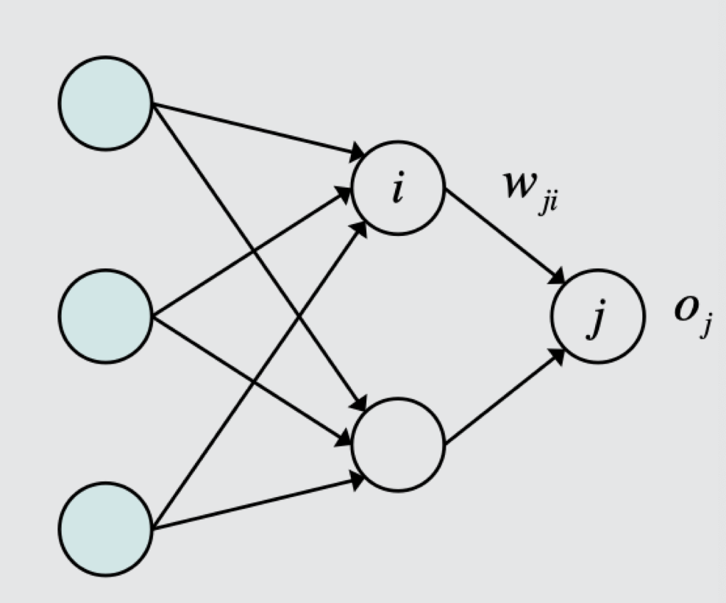
Notation of the network
$w_{ji}$: weights from perceptron i to j.
$o_j$: output of perceptron j, taking activation function of $net_j$.
$net_j$: input value of perceptron j.

Algorithm

• We first notice that each weight is changed by

  \[\begin{aligned} \Delta w_{ji} &= -\eta \frac{\partial E}{\partial w_{ji}} \\ &= -\eta \frac{\partial E}{\partial net_j}\frac{\partial net_j}{\partial w_{ji}} \\ &= -\eta\frac{\partial E}{\partial net_j}o_i \end{aligned}\]
  • Notice that $o_i$ can be replaced by $x_i$ if $i$ is an input perceptron. Recall that $net(w_i) = w_0 + \sum_{i=1}^n w_ix_i$, $\frac{\partial net_j}{\partial w_{i}} = x_i$.
  • For easy understanding, we use $\delta_j$ to denote $\frac{\partial E}{\partial net_j}$, that is $\delta_j =\frac{\partial E}{\partial net_j}$

• Next we want to calculate the $\delta_j$, there are two situations, where j is an output perceptron or not.

  • j is an output perceptron.

    \[\begin{aligned} \delta_j &= \frac{\partial E}{\partial o_j}\frac{\partial o_j}{\partial net_j}\\ &= \frac{\partial o_j}{\partial net_j}(o_j-y_j) \end{aligned}\]

  • j is a hidden perceptron.

    \[\begin{aligned} \delta_j &= \frac{\partial o_j}{\partial net_j}\sum_k \delta_k w_{kj} \end{aligned}\]

More Illustration of Backpropagation

Gradient descent with Backpropagation

1. Initialize Network with Random Weights and Biases.
2. For each Training Image:
   1. Compute Activation for the Entire Network.

   2. Compute $\delta = \frac{\partial E}{\partial net_j}$ for Neurons in the Output Layer using Network Activaion and Desired Activation.

      \[\begin{aligned} \delta_j^{(L)} &= \frac{\partial E}{\partial net_j}\\ &= \frac{\partial E}{\partial o_j}\frac{\partial o_j}{\partial net_j}\\ &= \frac{\partial o_j}{\partial net_j}(o_j-y_j) \end{aligned}\]

   3. Compute $\delta = \frac{\partial E}{\partial net_j}$ for all Neurons in the previous Layers (Hidden Perceptron). To be noticed, $l+1$ denotes the previous layer of layer $l$. $k$ denotes the $k$th percepton in a single layer $l$.

      \[\begin{aligned} \delta_j^{(l)} &= \frac{\partial E}{\partial net_j}\\ &= \frac{\partial o_j}{\partial net_j}\sum_k \delta_k^{l+1} w_{kj}^{l+1} \end{aligned}\]

   4. Compute Gradient of Cost w.r.t each Weight and Bias for the Training Image using $\delta$

      \[\begin{aligned} \frac{\partial E}{\partial w_{jk}^{(l)}} &= \frac{\partial E}{\partial net_j}\frac{\partial net_j}{\partial w_{jk}^{(l)}} \\ &= \delta_j^{(l)}o_k^{(l-1)} \end{aligned}\] \[\begin{aligned} \frac{\partial E}{\partial b_{j}^{(l)}} &= \frac{\partial E}{\partial net_j}\frac{\partial net_j}{\partial b_{j}^{(l)}} \\ &= \delta_j^{(l)} \cdot 1 = \delta_j^{(l)} \end{aligned}\]

3. Average the Gradient w.r.t. each Weight and Bias over the Entire Training Set (Assume total $n$ samples).

   \[\begin{aligned} &\frac{\partial E}{\partial w_{jk}^{(l)}} = \frac{1}{n}\sum\frac{\partial E}{\partial w_{jk}^{(l)}}\\ &\frac{\partial E}{\partial b_{j}^{(l)}} = \frac{1}{n}\sum\frac{\partial E}{\partial b_{j}^{(l)}} \end{aligned}\]

4. Update the Weights and Biases using Gradient Descent.

   \[\begin{aligned} w_{jk}^{(l)} &= w_{jk}^{(l)} + \Delta w_{jk}^{(l)} \\ &= w_{jk}^{(l)} + (-\eta \frac{\partial E}{\partial w_{ji}}) \end{aligned}\] \[\begin{aligned} b_{j}^{(l)} &= b_{j}^{(l)} + \Delta b_{j}^{(l)} \\ &= b_{j}^{(l)} + (-\eta \frac{\partial E}{\partial b_{j}^{(l)}}) \end{aligned}\]
5. Repeat Steps 2-4 till Cost reduces below an acceptable level (Convergence)