Support Vector Machines
Motivation
Linear classification usually assume perfect separation between the two classes. However, if a new data point is introduced to the system, the current linear model may not be able to capture it. Therefore, the margin is introduced to address this problem.
Margin
Lemma 1
$x$ has distance $\frac{|f_w(x)|}{||w||}$ to the hyperplane $f_w(x) = w^Tx = 0$.
Proof:
$w$ is orthogonal to the hyperplane. (点法式)
The unit direction is $\frac{w}{||w||}$
The projection of $x$ is $(\frac{w}{||w||})^Tx = \frac{f_w(x)}{||w||}$
Remarks:
Proof of the distance of a given point $Q$($x_0$, $y_0$, $z_0$) to a given hyperplane $Ax+Bx+Cx+D=0$, or say $w^Tx+D=0$. To simplify the calculation, we use 3 dimension space.
Take a randomly pick point $P$($x$, $y$, $z$) located on the plane. Build a normal vector $\vec{n}$ = ($A$, $B$, $C$) = $w$ cross the point $P$. And we can easily think of that the distance of $Q$ and the plane is just the length of the projection of $Q$ on the $\vec{n}$. Therefore, we have
\[\begin{aligned} d &= |\vec{PQ}| \cdot \cos{\theta}\\ &= \frac{|\vec{n}|}{|\vec{n}|} \cdot |\vec{PQ}| \cdot \cos{\theta} \\ &= \frac{|\vec{n}|\cdot |\vec{PQ}| \cdot \cos{\theta}}{|\vec{n}|} \\ &= \frac{A(x_0-x) + B(y_0-y) + C(z_0-z)}{\sqrt{A^2 + B^2 + C^2}} \\ &= \frac{Ax_0 + By_0 + Cz_0 - (Ax + By + Cz)}{\sqrt{A^2 + B^2 + C^2}} \\ &= \frac{Ax_0 + By_0 + Cz_0 + D}{\sqrt{A^2 + B^2 + C^2}} \\ &= \frac{f_w(x)}{||w||} \end{aligned}\]$|\vec{A}|\cdot |\vec{B}| \cdot \cos{\theta}$ is just the projection of vector A on the vector B
$PQ = (x_0-x, y_0-y, z_0-z)$
Since P located on the plane, thus $Ax + By + Cz + D = 0$.
Claim 1
$w$ is orthogonal to the hyperplane $f_{w,b}(x) = w^Tx+b = 0$.
Claim 2
$0 (0,0,0)$ has distance $\frac{|b|}{||w||}$ to the hyperplane $f_{w,b}(x) = w^Tx+b = 0$.
Lemma 2
$x$ has distance $\frac{f_{w,b}(x)}{||w||}$ to the hyperplane $f_{w,b}(x) = w^Tx+b = 0$.
Proof:
Let $x = x_a + r\frac{w}{||w||}$, then |r| is the distance, $x_a$ locates on the plane.
Thus, we prove that $r = \frac{f_{w,b}(x)}{||w||}$. $f_{w,b}(x_a) = 0$ is because $x_a$ locates on the plane.
Support Vector Machine (SVM)
Objective
- Margin over all training data points:
\(\gamma = \min_{i}\frac{|f_{w,b}(x_i)|}{||w||}\) - Only want correct $f_{w,b}$, and $y_i \in {+1, -1}$, we have,
\(\gamma = \min_{i}\frac{y_if_{w,b}(x_i)}{||w||}\) - If $f_{w,b}$ incorrect on some, the margin is negative.
- Maximize margin over all training data points: \(\max_{w,b}\gamma = \max_{w,b}\min_i \frac{y_if_{w,b}(x_i)}{||w||} = \max_{w,b}\min_i \frac{y_i(w^Tx_i +b)}{||w||}\)
Simplified Objective
Claim 1
When $(w,b)$ scaled by a factor $c$, the margin won’t change, that is
Therefore, we can consider a fixed scale such that
\[y_{i*}(w^Tx_{i*} + b) = 1\]where $x_{i*}$ is the point closet to the hyperplane. Therefore, for all other data, we have,
\[y_{i*}(w^Tx_{i*} + b) \geq 1\]The margin thus is $\frac{1}{\lvert\lvert w \rvert\rvert}$, and the optimization can be simplified to
\[\begin{aligned} & \begin{cases} &\max \min_{w,b}\frac{y_{i}(w^Tx_{i} + b)}{||w||}\\ &y_i(w^Tx_i+b) \geq 1, \forall i \end{cases}\\ \rightarrow&\begin{cases} &\max_{w,b} \frac{1}{||w||}\min_{x_i}y_{i}(w^Tx_{i} + b)\\ &y_i(w^Tx_i+b) \geq 1, \forall i \end{cases}\\ \rightarrow&\begin{cases} &\max_{w,b} \frac{1}{||w||}\min_{x_i*}y_{i*}(w^Tx_{i*} + b)\\ &y_i(w^Tx_i+b) \geq 1, \forall i \end{cases}\\ \rightarrow&\begin{cases} &\max_{w,b} \frac{1}{||w||} \cdot 1\\ &\min y_{i*}(w^Tx_{i*}+b) = 1, \forall i \end{cases}\\ \rightarrow&\begin{cases} &\min_{w,b}\frac{1}{2}||w||^2\\ &y_i(w^Tx_i+b) \geq 1, \forall i \end{cases}\\ \end{aligned}\]To be notice, $\min y_{i}(w^Tx_{x_i}+b) = 1$ has the same meaning as the $y_i(w^Tx_i+b) \geq 1$ Therefore, we want to minimize the $\frac{1}{2}||w||^2$.
Remarks: Maximum margin classifier means that we want to find the margin that can maximize the smallest distance to the margin. Can think like this way, when you are walking on a road where both sides of the road are cliff, the safest location must be the center of the road.
Lagrange Multiplier
To solve the aforementioned minimization problem, we will introduce the application of lagrangian.
Lagrangian
Consider optimization problem:
We have lagrangian:
\[\mathcal{L}(w, \beta) = f(w) + \sum_{i}\beta_ih_i(w)\]where $\beta_i$ are called lagrange multipiler. Can be solved by setting derivatives of Lagrangian to 0.
\[\frac{\partial{\mathcal{L}}}{\partial{w_i}} =0; \,\,\frac{\partial{\mathcal{L}}}{\partial{\beta_i}} =0\]Generalized Lagrangian
Consider optimization problem:
Generalized Lagrangian:
\[\mathcal{L}(w, \beta) = f(w) + \sum_{i}\alpha_ig_i(w) + \sum_{j}\beta_jh_j(w)\]Consider the quantity:
\[\theta_p(w) := \max_{\alpha, \beta:\alpha_i \geq 0} \mathcal{L}(w, \alpha, \beta)\]According to the aformention s.t. condition, minimizing $f(w)$ is the same thing as minimizing $\theta_p(w)$
\[\min_wf(w) = \min_w\theta_p(w) = \min_w\max_{\alpha, \beta:\alpha_i \geq 0} \mathcal{L}(w, \alpha, \beta)\]Lagrange duality
The primal problem
The dual problem
\[d^* := \max_{\alpha, \beta:\alpha_i \geq 0}\min_w \mathcal{L}(w, \alpha, \beta)\]Karush-Kuhn-Tucker (KKT) conditions
Under KKT conditions, there exists $(w, \alpha, \beta)$ such that
Following is the KKT condition:
\[\begin{cases} &\frac{\partial{\mathcal{L}}}{\partial{w_i}} = 0 \\ &\alpha_ig_i(w) = 0 \,\,\,\,(Dual\,\, complementarity)\\ & g_i(w)\leq0, \,\,h_j(w)=0 \,\,\,\,(Primal\,\, constraints)\\ & \alpha_i \geq 0 \,\,\,\,(Dual\,\, constraints) \end{cases}\]SVM Optimization
Recall the optimization problem,
\[\begin{cases} &\min_{w,b}\frac{1}{2}||w||^2\\ &y_i(w^Tx_i+b) \geq 1, \forall i \end{cases}\]We have the generalized Lagrangian
\[\mathcal{L}(w,b,\alpha) = \frac{1}{2}||w||^2 - \sum_{i}\alpha_i[y_i(w^Tx_i+b) -1]\]where $\alpha$ is the lagrange multiplier.
Next, we want to check the KKT conditions:
Notice, $\frac{\partial{w^TB}}{\partial w} = B$
Plug into $\mathcal{L}$, we have
Therefore, the problem is reduced to a dual problem,
\[\begin{aligned} \mathcal{L}(w,b,\alpha) &= \sum_i\alpha_i - \frac{1}{2}\sum_{ij}\alpha_i\alpha_jy_iy_jx_i^Tx_j \\ &\sum_i\alpha_iy_i = , \,\,\alpha_i \geq 0 \end{aligned}\]Since $w = \sum_i\alpha_iy_ix_i$, we have $w^Tx+n = (\sum_i\alpha_iy_ix_i^T)x+b$, only depend on inner products $x_i^Tx_j$
Support Vectors
- Final solution is a sparse linear combination of the training instances.
- Those instances with $\alpha_i > 0$ are called support vectors, these instances lie on the margin boundary.
- Solution not changed if delete the instances with $\alpha_i=0$
Learning Theory Justification
To minimize the VC dimension leads to maximize the margin.
Variants: Soft-margin and SVR
Soft-margin SVM
Recalled Hard-margin SVM,
However, if the training instances are not linearly separable, hard-margin will fail. Therefore, to address this problem, slack variables (denoted by $\xi_i$) are introduced to tolerate errors.
We have soft-margin SVM,
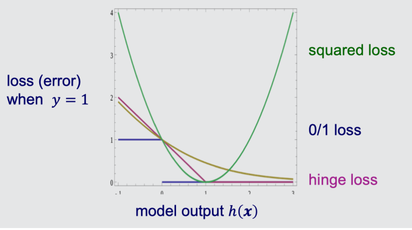
$C$ determines the relative importance of maximizing margin vs. minimizing slack. $\zeta_i$ is the hinge loss.
Hinge Loss
Different from minimizing squared loss and cross-entropy loss, SVMs minimize hinge loss.
Definition of hinge loss in SVM, y is the label, i.e. $\pm 1$
Support Vector Regression
Overview
- the SVM idea can also be applied in regression tasks
- an $\epsilon$-insensitive error function specifies that a training instance is well explained if the model’s prediction is within $\epsilon$ of $y_i$
- Regression using slack variables (denoted by $\zeta_i$, $\xi_i$) to tolerate errors. We have Support Vector Regression
Slack variables allow predictions for some training instances to be off by more than $\epsilon$.
Kernel Method
Idea
A proper feature mapping can make non-linear to linear.
Recalled the SVM dual form, the $x_i^Tx_j$ can be replaced by $\phi(x_i)^T\phi(x_j)$, where ${\phi(x_i)}$ denotes a feature space that SVM will be applied. To be noticed, we don’t need to design $\phi(\cdot)$, only need to design the kernel, $k(x_i,x_j) = \phi(x_i)^T\phi(x_j)$
Polynomial kernels
Fix degree $d$ and constant $c$:
An example of polynomial kernels,
\[\forall x, x' \in \mathbb{R}^2, K(x,x') = (x_1x_1' + x_2x_2'+c)^2 = \begin{bmatrix} &x^2_1 \\ &x^2_2 \\ &\sqrt{2}x_1x_2 \\&\sqrt{2c}x_1 \\&\sqrt{2c}x_2 \\& c \end{bmatrix} \cdot \begin{bmatrix} &x'^2_1 \\ &x'^2_2 \\ &\sqrt{2}x'_1x'_2 \\&\sqrt{2c}x'_1 \\&\sqrt{2c}x'_2 \\& c \end{bmatrix}\]Gaussian/Radial Basis Function(RBF) kernels
- Fix bandwidth $\sigma$:
\(k(x,x') = exp(\frac{-||x-x'||^2}{2\sigma^2})\) - Un-normalized version
\(k'(x,x') = exp(\frac{x^Tx'}{\sigma^2})\) - Power series expansion
\(k'(x,x') = \sum_{i}^{+\infty}\frac{(x^Tx')^i}{\sigma^ii!}\) - Mercer’s condition for kernels
$k(x, x’)$ has expansion.
\(k(x, x') = \sum_i^{+\infty}\alpha_i\phi(x)\phi(x')\)
if and only if for any function $c(x)$,
\(\int\int c(x)c(x')k(x,x')dxdx'\geq0\)
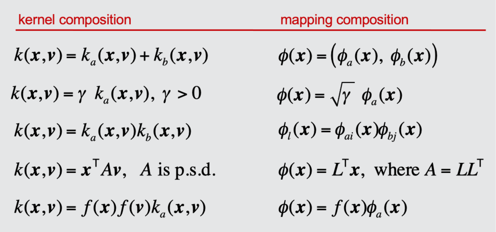
Kernels Algebra
Kernels are closed under positive scaling, sum, product, pointwise limit, and composition with a power series $\sum_i^{+\infty}\alpha_ik^i(x,x’)$.